After the training phase, we obtain estimates of the beta parameters of the
linear model. Given the beta values and the independent variables of the
training data, we can easily calculate the corresponding fitted values y_hat
for the training data: y_hat = beta_0 + beta_1 * x_1 + beta_2 * x_2 + ... +
beta_p x_p.
However, if a different training set were used, we would get a different set of beta values and hence y_hat values. We would expect them to be close to the previous set of beta values and of y_hat. More generally, if we repeated the training many times, with different training data, we would get a distribution (scattering) of each beta value. If we make some assumptions about the shape of that distribution, we can predict its spread for each of beta_0, beta_1, ... This spread is usually quoted as a confidence interval.
The confidence interval is a prediction, so it is expressed in terms of probability. For example, we might have found that beta_0 = 1.4 for the training data we were given. After calculating the confidence interval, we might predict, with 95% confidence, that beta_0 lies between 0.9 and 1.9 (say). This means that, if we were to repeat the training phase many times with different training data, the estimated beta_0 would lie in the range 0.9 to 1.9 95% of the time.
Because of the way it is calculated (with the assumption that the distribution is symmetric, etc.), the confidence interval is centred on the given estimate of beta, but there are other techniques that make weaker assumptions about how beta is distributed so the confidence interval would be different, but it will still be expressed as an interval and probability.
Generally, smaller (tighter) confidence intervals are better, because we have less uncertainty regarding the "true" value of the quantity (beta in this case).
One of the main uses of confidence intervals is to compare different models (having different predictors). If a confidence interval includes zero, it could be argued that the corresponding predictor might as well be zero and hence does not contribute to the model. Also, if two predictor variables are highly correlated, the confidence intervals for each will typically be very large. The two variables should be removed from the model and possibly replaced with a single variable that captures their combined effect. Its associated beta would have a smaller confidence interval than if the other variable were also included in the model.
Lastly, confidence intervals can be calculated for both the beta and y_hat
values.
Confidence limits give us a way to quantify the uncertainty in a) the model parameters discovered from the training data. We can also propagate that uncertainty to the predicted values.
The purpose of adding more training data is to reduce the uncertainty in the fitted parameters and hence in the predicted values for the test set.
Interestingly, we can predict the value of each additional training observation (row in the dataframe) by calculating the Fisher Information Matrix for a given model and dataset combination. This is an advanced topic and is not covered in this module. But students should be aware that there is a way of "scoring" the value of the training data, which is obviously more valuable at times when observations are difficulty to obtain. Typically, machine learning applications have lots of data, but the value of individual observations might be low, and this can be "measured" using the Fisher Information Matrix.
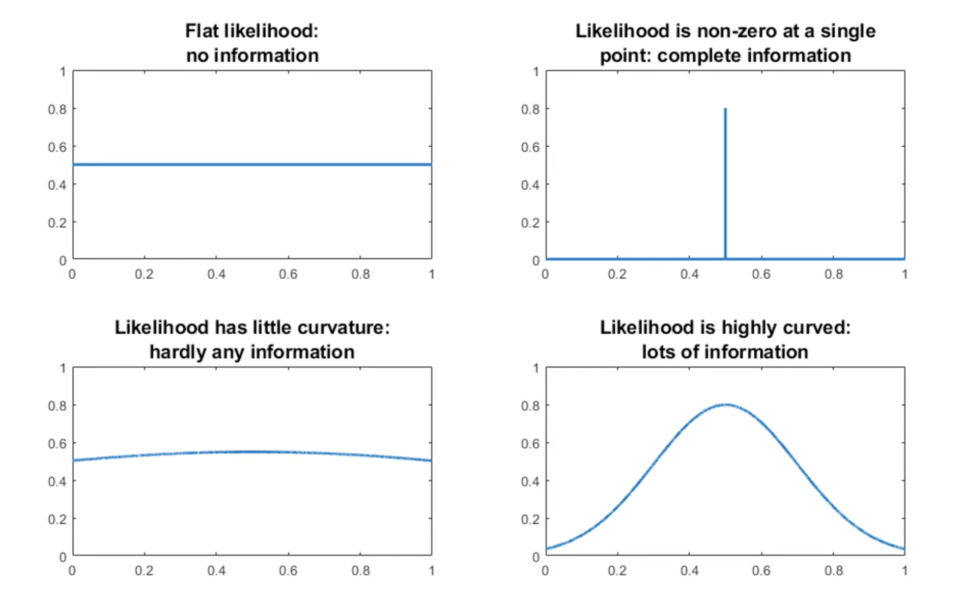
Source: Statlect
Referring to the plots above, the Fisher information captures the extent to which the parameters predict the training data. If the Fisher Information is low, the parameter values have little effect: any of a wide range of parameters values would predict the data just as well. This is another way of saying that the model is not very effective.
For python, statsmodels offers a suitable function to compute the information matrix.
Scikit-learn offers excellent guidance on regression metrics.